


Radiocarbon Dating Basics
Radiocarbon (carbon-14)
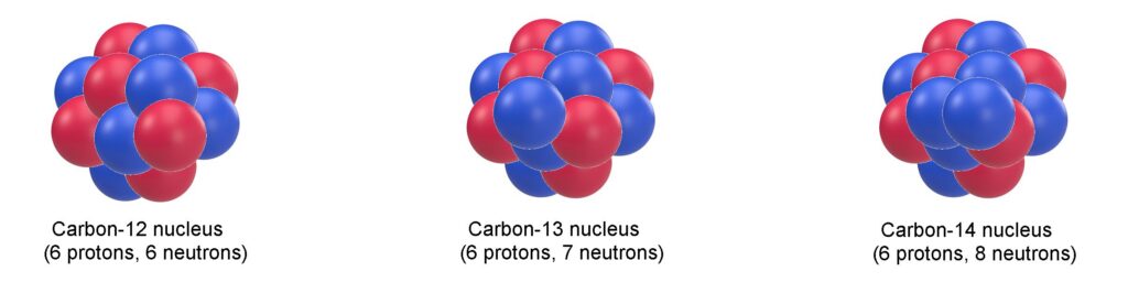
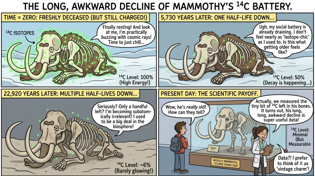
There are three naturally-occurring isotopes of carbon; carbon-12 (¹²C), carbon-13 (¹³C) and carbon-14 (¹⁴C). ¹⁴C is a radioactive isotope of carbon that contains six protons (that’s what makes it carbon) and eight neutrons, giving it an atomic mass of 14. Unlike the stable isotopes ¹²C and ¹³C, which make up approximately 99% and 1% of natural carbon respectively, ¹⁴C exists only in trace amounts and is continuously produced in the Earth’s upper atmosphere through the interaction of cosmic rays with nitrogen atoms. While ¹²C and ¹³C are stable and do not decay, ¹⁴C undergoes beta decay with a half-life of about 5,700 years (Kondev 2021), transforming into nitrogen-14 (¹⁴N) over time.
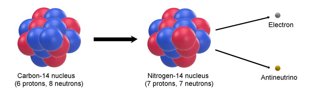
This radioactive decay makes ¹⁴C especially useful for radiocarbon dating, allowing scientists to determine the age of formerly living materials by measuring the remaining ¹⁴C content relative to the stable isotopes.
Carbon-14 is formed in the upper atmosphere when high-energy cosmic rays collide with nitrogen-14 (¹⁴N) atoms, triggering a nuclear reaction that converts the nitrogen into radioactive carbon-14. This newly formed ¹⁴C quickly oxidizes to carbon dioxide and becomes incorporated into the global carbon cycle, entering plants, animals, and eventually sediments. The rate of ¹⁴C production fluctuates slightly due to changes in solar activity and variations in Earth’s geomagnetic field. Increased solar activity strengthens the solar wind and magnetic field, which deflects cosmic rays and reduces ¹⁴C formation, while a weaker geomagnetic field allows more cosmic rays to penetrate the atmosphere, enhancing production.
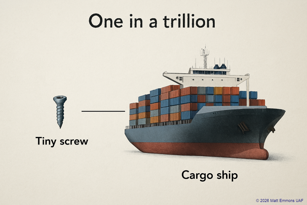
To give some idea of the tiny amount of carbon-14 present in the atmosphere, consider the following:
-
Approximately one atom in a trillion atoms of atmospheric carbon is carbon-14
-
Approximately 1.2 x 10⁻¹² of atmospheric carbon is carbon-14
-
The amount of carbon-14 in the atmosphere is equivalent to a single grain of salt in a full railroad hopper car (a standard hopper car holds about 100 tons)
-
The amount of carbon-14 in the atmosphere is equivalent to one drop of water in 20 Olympic swimming pools (an Olympic pool contains about 2.5 million liters)
-
The amount of carbon-14 in the atmosphere is equivalent to one second in about 31,700 years.
All images created by Matt Emmons
Isotope Ratios (digression)
Stable Isotopes in Environmental, Biological, and Earth System Research
Stable isotopes are non‑radioactive isotopes whose relative abundances vary predictably as a result of physical, chemical, and biological processes. These variations expressed as isotope ratios (e.g., δ¹³C, δ¹⁵N) are powerful tracers of environmental conditions, geographic origin, and ecological relationships. Because stable isotopes fractionate during processes such as evaporation, photosynthesis, metabolism, and mineral formation, their ratios encode information about both place and process.
Carbon Isotopes (¹²C / ¹³C)
Carbon isotopes are foundational to studies of carbon cycling, ecology, and paleoenvironments. Variations in δ¹³C primarily reflect photosynthetic pathway and carbon source. C₃ plants (most trees and temperate vegetation) are isotopically lighter than C₄ plants (such as grasses and maize), while CAM plants occupy an intermediate range. These differences propagate through food webs, allowing δ¹³C to be used to reconstruct diet, trophic structure, and vegetation change.
Geographically, δ¹³C varies as a function of vegetation type, aridity, and atmospheric CO₂ conditions. At higher trophic levels, carbon isotope values shift only modestly, preserving strong signals of basal carbon sources and enabling differentiation between terrestrial, freshwater, and marine food webs.
Nitrogen Isotopes (¹⁴N / ¹⁵N)
Nitrogen isotopes are especially informative for understanding trophic position and nitrogen cycling. δ¹⁵N values systematically increase (typically by 3–5‰) with each trophic level due to preferential excretion of ¹⁴N during metabolism. This makes nitrogen isotopes a core tool in food‑web reconstruction, paleoecology, and archaeology.
Geographic variability in δ¹⁵N reflects differences in soil processes, precipitation, aridity, and nutrient cycling, including microbial activity such as denitrification. Marine systems often show elevated baseline δ¹⁵N values compared to terrestrial systems, and anthropogenic inputs (e.g., fertilizers, sewage) can leave distinct isotopic signatures in modern and archaeological contexts.
Oxygen Isotopes (¹⁶O / ¹⁸O)
Oxygen isotopes are key tracers of climate, hydrology, and temperature. Variations in δ¹⁸O arise from fractionation during evaporation and condensation, creating systematic geographic patterns tied to latitude, altitude, distance from the coast, and temperature. As a result, oxygen isotopes form the basis of isoscapes used to infer geographic origin of water, organisms, and materials.
In biological tissues and carbonates (e.g., shells, speleothems, tooth enamel), δ¹⁸O records the isotopic composition of ambient water modified by temperature‑dependent fractionation, enabling reconstruction of paleoclimate, seasonality, and mobility.
Hydrogen Isotopes (¹H / ²H, Deuterium)
Hydrogen isotopes parallel oxygen isotopes in many respects and are strongly controlled by the hydrologic cycle. δ²H values vary predictably with latitude, elevation, and continentality, and are widely used to track water sources, animal migration, and moisture pathways.
In ecological and forensic research, hydrogen isotopes in keratinous tissues (hair, feathers) or plant waxes provide insights into geographic origin and movement. Because hydrogen in organic matter reflects both environmental water and metabolic effects, interpretation typically benefits from combined multi‑isotope approaches.
Sulfur Isotopes (³²S / ³⁴S)
Sulfur isotopes are valuable tracers of redox conditions, marine influence, and sulfur cycling. δ³⁴S values differ markedly between marine sulfate, terrestrial sulfate, sulfide minerals, and biogenic sulfur. Coastal and marine ecosystems often exhibit elevated δ³⁴S values compared to inland systems, allowing sulfur isotopes to distinguish between marine and terrestrial inputs in diets, sediments, and biological tissues.
Sulfur isotopes do not fractionate strongly across trophic levels, making them particularly useful for identifying basal sulfur sources rather than trophic position.
Geographic and Trophic Structuring of Stable Isotopes
Across all stable isotopes, two fundamental organizing principles apply:
- Geographic structuring arises from climate, geology, and hydrology, producing spatially coherent isotopic patterns (“isoscapes”).
- Trophic structuring arises from biological fractionation during metabolism, most strongly expressed in nitrogen and, to a lesser extent, carbon isotopes.
Together, these principles allow stable isotope data to be used in ecology, archaeology, paleoclimate reconstruction, food authentication, hydrology, and forensic science, especially when multiple isotopic systems are combined.
Radiogenic Isotopes and Their Use in Dating and Chronology
In contrast to stable isotopes, radiogenic isotope systems involve the decay of unstable parent isotopes into stable daughter isotopes at known rates. These decay systems form the basis of absolute dating methods that constrain the timing of geological, archaeological, and planetary processes over timescales ranging from thousands to billions of years.
Radiogenic isotope dating differs fundamentally from stable isotope analysis in that the information derives from time‑dependent radioactive decay, not fractionation.
Carbon‑14 (¹⁴C) Dating
Radiocarbon dating exploits the radioactive decay of ¹⁴C to ¹⁴N and is used to date organic and carbonate materials formed within approximately the last 50,000 years. Because ¹⁴C is produced in the atmosphere and incorporated into living systems, radiocarbon ages reflect the time since biological carbon exchange ceased. This method underpins chronology in archaeology, paleoecology, climate science, and environmental studies.
Uranium‑Series Dating (U–Th)
Uranium‑series methods rely on the decay of uranium isotopes (²³⁸U, ²³⁵U) to thorium isotopes and are widely used to date carbonates such as corals, speleothems, and travertines. Because uranium is soluble and thorium is not, newly formed carbonates incorporate uranium but exclude thorium, allowing age determination based on daughter ingrowth. U–Th dating extends far beyond the range of radiocarbon and provides high‑precision ages for Quaternary records.
Potassium–Argon and Argon–Argon (K–Ar, ⁴⁰Ar/³⁹Ar)
These systems date materials based on the radioactive decay of ⁴⁰K to ⁴⁰Ar and are essential for dating volcanic rocks and ash layers. Argon–argon dating allows high‑precision incremental heating and cross‑calibration, forming a cornerstone of geological time scales and stratigraphic correlation.
Rubidium–Strontium and Samarium–Neodymium (Rb–Sr, Sm–Nd)
These long‑lived decay systems are widely used to date igneous and metamorphic rocks and to trace crust–mantle evolution. Because isotopic ratios evolve predictably over time, they are also used as geochemical tracers of source regions, not just chronological tools.
Lead Isotopes (Pb–Pb)
Lead isotope systems are used both for dating and for provenance studies. Because different decay chains produce different lead isotopes, lead isotope ratios can constrain the age of ore formation and trace contamination pathways in environmental investigations.
Summary: Complementary Roles of Stable and Radiogenic Isotopes
Together, stable and radiogenic isotopes form a complementary toolkit:
- Stable isotopes reveal processes, environments, and biological interactions through fractionation.
- Radiogenic isotopes provide time constraints through predictable radioactive decay.
In modern research, these approaches are often integrated, for example combining radiocarbon chronology with stable isotope paleoecology to produce robust, multi‑dimensional reconstructions of the Earth system and human-environment interactions over time.
The Radiocarbon Curve
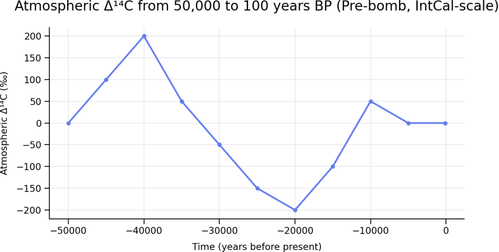
The plot shown above represents the changes in atmospheric concentration of carbon-14 over the last 50,000 years derived from the IntCal calibration framework data. The y‑axis (Δ¹⁴C, per mil) shows the relative deviation of atmospheric ¹⁴C/¹²C from modern, corrected for radioactive decay. The plot does not include the ‘post-bomb’ carbon-14 contamination, in other words it covers from 50,000 year ago until just before the 1950’s nuclear bomb testing.
How little atmospheric ¹⁴C has changed over this interval
Despite spanning nearly 50,000 years, the atmospheric ¹⁴C concentration has remained remarkably constrained:
- Δ¹⁴C variations are largely confined to a range of roughly −200‰ to +200‰, even during major climate events such as glacial–interglacial transitions.
- These fluctuations reflect changes in cosmic ray flux, geomagnetic field strength, ocean circulation, and carbon exchange rates, not wholesale changes in atmospheric composition.
- In absolute terms, this corresponds to small percentage changes in atmospheric ¹⁴C abundance, especially when contrasted with the dramatic spike caused by mid‑20th‑century nuclear testing (+800–1000‰).
- For most of the Late Pleistocene and Holocene, atmospheric ¹⁴C has behaved as a quasi‑steady tracer, oscillating but remaining well mixed and globally coherent.
This long‑term stability is precisely what makes radiocarbon dating viable. The method relies on the fact that, prior to the bomb period, atmospheric ¹⁴C varied slowly, smoothly, and within well‑characterized limits, allowing calibration curves like IntCal to correct for these modest deviations with high confidence.
Here is the plot showing how atmospheric carbon‑14 (Δ¹⁴C) has changed over the last 100 years, including the nuclear weapons “bomb pulse”:
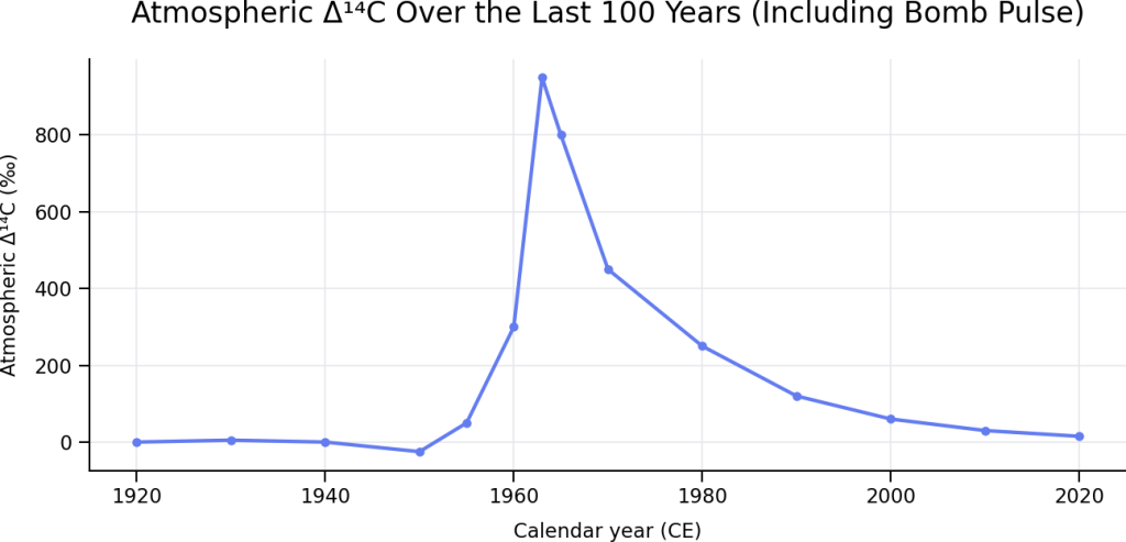
This figure highlights a fundamental contrast with the long‑term behavior you saw in the earlier 50,000‑year plot.
Pre‑bomb stability (ca. 1920–1950)
- From the early 20th century until ~1950, atmospheric Δ¹⁴C fluctuated only slightly around 0‰ to −25‰.
- These small variations reflect natural processes such as changes in solar activity, geomagnetic field strength, and carbon exchange between the atmosphere, oceans, and biosphere.
- This range is entirely consistent with the modest variability seen throughout the Holocene and late Pleistocene.
The bomb pulse (1950s–early 1960s)
- Atmospheric nuclear weapons testing abruptly doubled the amount of radiocarbon in the atmosphere.
- Δ¹⁴C values rose from slightly negative to nearly +1000‰ by 1963, the highest atmospheric ¹⁴C concentrations observed in the last tens of thousands of years.
- This increase occurred over less than a decade, making it unprecedented in both magnitude and rate.
Post‑bomb decline (mid‑1960s to present)
- Following the Limited Test Ban Treaty (1963), atmospheric Δ¹⁴C began a steady decline.
- Excess ¹⁴C has been absorbed by oceans, soils, vegetation, and the deep biosphere, a process that continues today.
- Despite this decline, modern atmospheric Δ¹⁴C remains well above pre‑1950 levels, still carrying a strong bomb‑derived signal.
Why this plot matters
- The entire bomb pulse spans nearly 1000‰, dwarfing the ±200‰ natural range characteristic of the previous 50,000 years.
- This dramatic contrast explains why post‑1950 samples must be treated separately in radiocarbon science and why “bomb carbon” enables high‑precision dating of modern materials (decadal to sub‑annual resolution).
- It also reinforces an important point: radiocarbon dating works because the atmosphere was remarkably stable before human intervention and demonstrably not stable afterward.
Radiocarbon Dating Limitations
Understanding the Limitations of Radiocarbon Dating
Radiocarbon dating is a powerful and widely used method for determining the age of carbon‑bearing materials, but like all scientific techniques, it has important limitations. Understanding these limitations helps ensure that radiocarbon results are interpreted correctly and that sample selection and research design are well matched to the method.
Finite Age Range
Radiocarbon dating is effective only within a limited time window. Because radioactive carbon decays over time, very old samples retain too little 14C to be measured reliably. In practice, radiocarbon dating is generally limited to materials younger than about 45,000–50,000 years. Ages approaching this limit often carry larger uncertainties and should be interpreted as minimum ages rather than precise calendar dates.
Radiocarbon Ages Must Be Calibrated
Radiocarbon measurements produce results in “radiocarbon years,” which are not the same as calendar years. Atmospheric 14C levels have varied through time due to changes in solar activity, the Earth’s magnetic field, and the global carbon cycle. As a result, all radiocarbon ages must be calibrated using internationally accepted calibration curves. In some periods, calibration produces multiple possible calendar-age ranges or reduced precision, even for high‑quality measurements.
Reservoir Effects
Radiocarbon dating assumes that a sample’s carbon reflects the 14C content of the atmosphere at the time it formed. This assumption is not always valid. Marine organisms, freshwater organisms, and some carbonates may incorporate carbon that is older than the atmosphere, causing samples to appear artificially old. These so‑called reservoir effects vary by location and environment and must often be corrected using independent data.
Sensitivity to Contamination
Radiocarbon dating is extremely sensitive to contamination. Very small amounts of carbon from soils, groundwater, conservation treatments, or modern handling can significantly affect results. While laboratory pretreatment removes many contaminants, it cannot always eliminate them completely. For this reason, careful sample selection and documentation of sample history are critical.
“Inbuilt Age” of Materials
Radiocarbon dating measures when carbon was fixed from the atmosphere, not necessarily when an object was used or deposited. For example, wood charcoal dates the time the tree ring grew, not when the wood was burned. Long‑lived materials may therefore appear older than the event of interest unless short‑lived components are targeted.
Mixing and Reworked Material
Many samples contain carbon from more than one source or time period. Sediment mixing, bioturbation, redeposition, or bulk sampling can result in age averaging, where the measured radiocarbon age does not correspond to a single event. Discrete, well‑defined materials usually produce the most meaningful results.
Post‑1950 “Bomb Carbon”
Atmospheric nuclear testing in the mid‑20th century dramatically increased 14C levels worldwide. As a result, samples formed after about 1950 require specialized calibration and may produce multiple possible calendar ages. While this “bomb carbon” can enable very precise dating of modern materials, it complicates interpretation when combined with older samples.
Material‑Specific Challenges
Not all materials are equally suitable for radiocarbon dating. Some materials consistently yield reliable results, while others are more prone to carbon exchange, contamination, or complex carbon sources. Each material type requires appropriate pretreatment and interpretive caution.
Interpretation Requires Context
Radiocarbon dating provides a measurement of a carbon‑bearing fraction, it does not automatically determine the age of an event. Archaeological, geological, or environmental context is essential for meaningful interpretation. Dates should always be evaluated alongside stratigraphy, association, and independent lines of evidence.
Summary
Radiocarbon dating is a robust and well‑established method, but its accuracy depends on appropriate sample selection, careful laboratory preparation, and informed interpretation. Understanding its limitations allows researchers and clients to ask the right questions, select the right materials, and use radiocarbon results with confidence. When applied thoughtfully, radiocarbon dating remains one of the most powerful tools for studying the recent past.
Radiocarbon Dating Units and Conventions
Overview
Radiocarbon ages measured by AMS are reported using a fairly standardized set of conventions so results are comparable across labs, time, and calibration software. These conventions cover how the age is expressed (units, reference year, half-life), what corrections are applied, and how calibrated ages are distinguished from raw radiocarbon ages. A widely endorsed summary of these conventions was published by (Millard 2014) and has become the current reference point for best practice.
Core Reporting Units and Basic Format
Conventional radiocarbon age
The primary way to report an AMS result is as a conventional radiocarbon age, expressed as:
- Format:
- Key conventions:
- Unit: 14C yr BP or ¹⁴C yr BP (not just “years BP”).
- BP definition: BP = “Before Present,” where “Present” is fixed as 1950 CE.
- Half-life used: The Libby half-life of 5568 years is used for conventional ages, even though the more accurate physical half-life is 5730 years (Kondev 2021) this maintains compatibility with the historical radiocarbon scale.
- Reference ratio: Ages are defined relative to a standard ¹⁴C/¹²C ratio that represents the atmosphere in 1950, assuming it was constant in the past (which is later corrected via calibration).
- Uncertainty:
- Reported as one standard deviation (1σ), combining counting statistics and other quantifiable sources of error.
- The age and error should typically be rounded consistently (e.g., to 10 years when the uncertainty is ≥ 10 years).
Millard recommends that every determination in a paper include, at minimum, a conventional radiocarbon age or a fraction modern (F¹⁴C) value with its uncertainty.
Fraction Modern (F¹⁴C) and Δ¹⁴C
For many AMS applications (especially recent carbon, atmospheric work, and reservoir studies), it is often more meaningful to report fraction modern and/or Δ¹⁴C instead of, or in addition to, a conventional age.
Fraction modern (F¹⁴C)
- Definition: F¹⁴C is the isotope ratio of the sample normalized to a standard “modern” reference, corrected for isotopic fractionation, where: F14C = 1.0 represents the 1950 atmospheric level of ¹⁴C.
- Format:
Dimensionless, but always explicitly labeled as F14C.
- Usage:
- Particularly important for post‑bomb samples, modern carbon cycle, and ocean/atmosphere studies, where “age” in years is less intuitive or even ambiguous.
Millard’s conventions explicitly state that either a conventional age in ¹⁴C yr BP or an F¹⁴C value (or both) should be reported for each determination, with fractionation correction stated or implied.
Δ¹⁴C
- Definition: Δ¹⁴C is the per mil deviation of a sample’s ¹⁴C content from the “modern” standard (1950 atmosphere), corrected for fractionation and decay since 1950.
- Format:
- Usage:
- Common in atmospheric monitoring, oceanography, and carbon cycle studies where relative enrichment or depletion is more relevant than a calendar age.
Isotopic Fractionation and δ¹³C Reporting
Radiocarbon measurements depend on ¹⁴C/¹²C, but that ratio is influenced by natural isotopic fractionation. Therefore, all conventional ages and F¹⁴C values are reported as being fractionation‑corrected, and the corresponding δ¹³C should be documented.
- δ¹³C format:
The reference scale (usually VPDB) should be stated.
- Role in reporting:
- The conventional radiocarbon age is defined as the age corresponding to a sample whose ¹⁴C/¹²C ratio has been normalized to δ¹³C = −25‰ (for terrestrial organic material).
- Labs usually either:
- Measure δ¹³C by IRMS and use it to correct the AMS ¹⁴C result.
- Or measure an “apparent δ¹³C” in the AMS system itself (less precise) if separate IRMS is not available.
- Best practice: Millard’s guidelines specify that the δ¹³C value actually used for fractionation correction should be reported along with the age or F¹⁴C value.
Calibration and Reporting of Calendar Ages
Raw AMS results (¹⁴C yr BP) do not directly equal calendar ages because atmospheric ¹⁴C has varied over time. Calibration curves and conventions for reporting calibrated ages are therefore crucial.
Calibration curves
- Current internationally accepted curves include:
- IntCal20 for the Northern Hemisphere.
- SHCal20 for the Southern Hemisphere.
- Marine20 for marine samples.
These curves are constructed from tree rings, corals, varves, and other archives, and are periodically updated.
Calibrated ages: formats and units
To avoid confusion between radiocarbon years and calendar years, clear distinctions in notation are used:
- Calibrated ages in years before present:
- Format:
cal BP or more explicitly “calibrated years BP”. - Example:
3820-3690 cal BP (95% probability, IntCal20)
- Format:
- Calendar years CE/BC (or AD/BC):
- Example:
- 2460–2280 cal BCE (95% probability, IntCal20)
- “cal” is kept to indicate the age is calibrated, and the curve used should be stated.
- Example:
- Key convention:
Millard notes that earlier conventions did not formally cover calibrated dates, and his updated guidelines explicitly recommend clearly distinguishing between conventional radiocarbon ages (¹⁴C yr BP) and calibrated calendar ages (cal BP, cal CE/BCE), and always stating which calibration curve and software were used.
Metadata and Contextual Information that Accompany AMS Ages
Millard’s conventions put a lot of emphasis on complete contextual reporting, not just the age number. For each radiocarbon determination in a scientific publication, the following should be provided wherever possible:
- Laboratory code:
- Example: OxA‑12345, AUR‑67890, etc.
- Allows traceability back to the lab and measurement.
- Sample material and context:
- Material: e.g., “charcoal”, “bone collagen”, “bulk peat”.
- Context: archaeological layer, stratigraphic unit, core depth, etc.
- Pretreatment method:
- e.g., ABA (acid–base–acid) for charcoal or collagen extraction protocol for bone.
- Important for assessing potential contamination and comparability.
- Measurement type and system:
- Indicate that the age was obtained by AMS (vs. gas or liquid scintillation counting).
- If relevant, instrument model and laboratory protocols can be referenced.
- Quality control measurements:
- Reference materials, blanks, and standards used to validate the run.
- Helps assess background and potential laboratory offsets.
- Calibration details (if calibrated ages are quoted):
- Calibration program (e.g., OxCal, CALIB, Bchron).
- Curve (IntCal20, SHCal20, Marine20).
- Probability range and level (typically 95%).
These details make the age reproducible, auditable, and interpretable for other researchers.
Accelerator Mass Spectrometer Measurements
Overview
The process by which the MiCaDaS performs radiocarbon analysis can be broken down into several sections that are described in detail in the following drop-down panels:
First, the graphite is ionized in the ion source. The ions produced (which also includes some iron, aluminum, nitrogen and oxygen ions) are extracted, focused and accelerated toward the low energy (LE) magnet.
The LE Magnet separates out many of the unwanted ions (aluminum, iron, oxygen) and directs ions in the mass range of 12 to 14 toward the accelerator.
The accelerator accelerates the ions and passes them through a region containing a small amount of helium gas. The ions ‘collide’ with the helium atoms and often lose an electron in the process (they are ‘stripped’ of electrons). The ions emerging from the other side of the accelerator are mostly singly-ionized carbon.
Next, the ion enter the magnetic field of the high energy magnet. This magnet separates carbon-12, 13 and 14 and directs them toward their own separate detectors.
Carbon-12 and carbon-13 are collected in their respective Faraday cup detectors located a short distance from the HE magnet and the carbon-14 ion beam continues toward the electrostatic analyzer (ESA).
The ESA helps to remove the few non-carbon-14 ions that managed to make their way through the instrument so far. After passing through the ESA, the ‘almost entirely’- carbon-14 ion beam continues toward the gas ionization detector (GID).
The GID detects the carbon-14 ions and can distinguish those very few ions that managed to get all the way through the instrument that weren’t carbon-14.
The measured quantities of the three carbon isotopes are then converted into 13C/12C and 14C/12C ratios.
Ion Source
A cesium sputter ion source is a specialized negative ion source used in AMS for producing negative ions from solid samples (e.g., graphite targets for radiocarbon dating). It relies on cesium vapor ionization and sputtering to liberate sample atoms and convert them into negative ions.
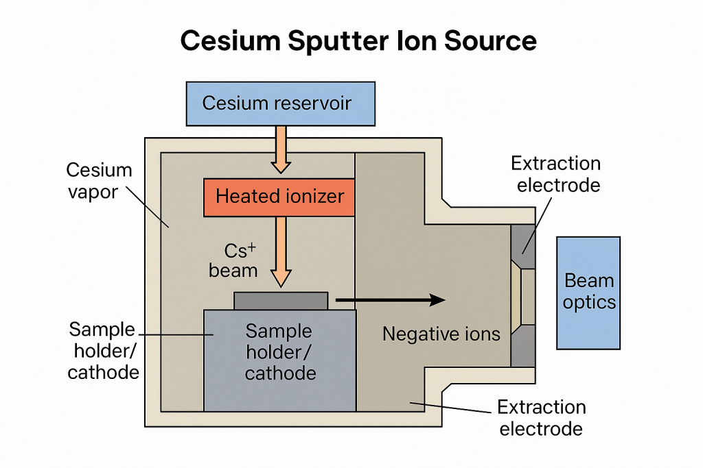
Key Components
- Cesium Reservoir: Contains metallic cesium, heated to produce cesium vapor.
- Heated Ionizer: A tungsten or tantalum surface heated to ~1000–1200 °C. Cesium vapor contacts the hot surface to produce Cs⁺ ions.
- Cs⁺ Beam: Cs⁺ ions are accelerated toward the sample cathode by an electric potential (typically 3–8 kV).
- Sample Holder / Cathode: Contains graphite or other sample material.
- Negative Ion Formation: Cs⁺ ions bombard the sample surface, sputtering atoms from the sample, Cesium bombardment also creates a high secondary electron density near the sample and some of the sputtered atoms capture electrons and form negative ions C⁻ .
- Extraction Electrodes: Pull negative ions out of the source at 20–35 kV.
- Beam Optics: Electrostatic lenses and apertures focus and steer the ion beam toward the AMS accelerator.
Low Energy Magnet
AMS instruments typically have two large magnets that separate ions of different masses. The one positioned immediately before the accelerator is called the low energy (LE) magnet and the one positioned immediately after is referred to as the high energy (HE) magnet. The LE magnet is configured so that only ions within or near the mass range of carbon (12 to 14 Daltons) enter the accelerator. All other ions produced from the ion source such as Iron (from the iron powder mixed with the graphite), aluminum (from the cathode) and oxygen will impact the internal surfaces of the instrument and are neutralized.
How a magnet separates ions of different mass
In a mass spectrometer with a magnetic sector, ions are first accelerated to (approximately) the same kinetic energy and then sent into a region with the magnetic field , usually perpendicular to their direction of motion. Charged particles moving through a magnetic field experience a force equal to the Lorenz Force given by
where q is the ion charge and v is its velocity. This force acts as the centripetal force resulting in the ions circular path, giving
rearranging for r the radius of curvature gives
If the ions enter the magnetic field with the same kinetic energy E (usually the case since a constant high voltage is usually employed to extract the ions from the ion source), then
rearranging for v
Substituting for v , we get
If E , q , and B are constant, then the radius of curvature is proportional to the square root of the mass.
By placing slits or Faraday cups at specific radii, the instrument collects or measures ions of only one mass (or mass window) at a time or on multiple detectors in parallel.
Electromagnets vs. Permanent Magnets
Historically, electromagnets were widely used because they allow adjustable field strength, which is useful for scanning across a range of masses. However, they require significant power and cooling systems. In contrast, modern instruments increasingly use permanent magnets, especially in compact or energy-efficient designs. These magnets offer excellent field stability, zero power consumption, and long-term reliability, making them ideal for continuous operation in isotope ratio mass spectrometry (IRMS) and accelerator mass spectrometry (AMS).
Faraday Cup Detector
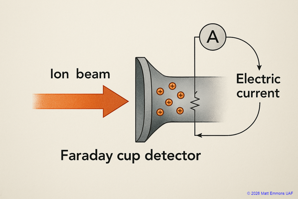
A Faraday Cup is a conductive metal cup designed to collect charged particles (usually positive ions in mass spectrometry). When ions strike the inner surface of the cup, they transfer their charge, generating a small measurable current proportional to the number of ions collected.
This principle is widely used in mass spectrometers, plasma diagnostics, particle beam systems, and space instrumentation.
Construction
Although variations exist, most FC detectors share a common structure:
- Metal cup or cylindrical collector: The main ion-collecting body.
- Entrance aperture: Allows ions to enter the cup while shielding it from stray signals.
- Electron‑suppression plate (or repeller): Prevents secondary electrons that are knocked out when ions hit the metal from escaping the cup, ensuring more accurate current readings.
- Grounded shield: Surrounds the assembly to eliminate external electrical interference.
- High‑value resistor to ground: Converts the ion-induced charge accumulation into a measurable voltage.
How the Faraday Cup Works
- Ions enter through the aperture and strike the inner metal surface of the cup.
- Secondary electrons are emitted, but the electron-suppression plate prevents them from escaping, ensuring the measurement reflects only incoming ion charge.
- The cup momentarily accumulates charge, which is discharged through a resistor, producing a tiny electric current.
- This current is amplified and converted to a voltage using high‑sensitivity electrometers.
- The measured current I is directly proportional to the number of ions hitting the detector (N is the number of ions per second and e is the elementary charge of 1.6 x 10⁻¹⁹ Coulombs):
Why Faraday Cups are Still Used Today
Despite the rise of more sensitive detectors, FCs remain indispensable because they provide:
- Highly accurate, absolute ion current measurement
- Mass‑independent detection (responds only to charge)
- Excellent long‑term stability
Accelerator and Stripper
While a standard mass spectrometer struggles to distinguish between isotopes of nearly identical mass (isobars), the accelerator uses brute-force physics to clear the noise and provide precision at the level of one-in-a-quadrillion.
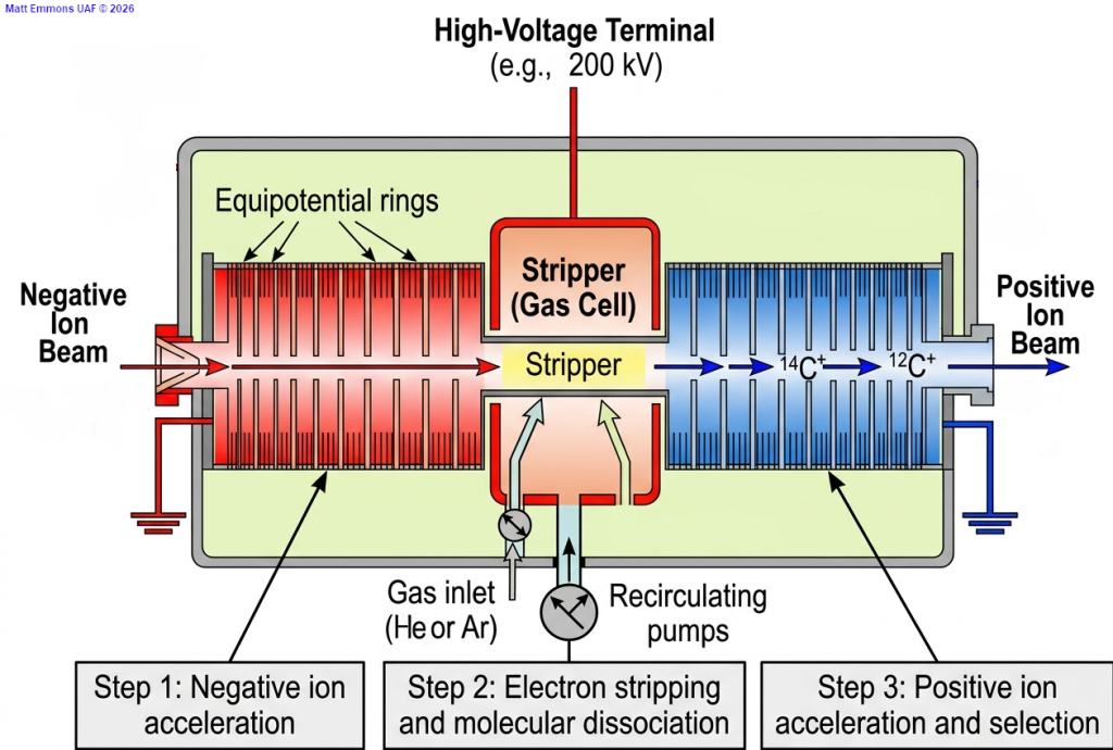
The Tandem Principle: One Voltage, Two Boosts
The genius of a tandem accelerator is that it uses a single high-voltage terminal to accelerate the ion beam twice. This is achieved by flipping the charge of the ions mid-flight.
- The process begins with negative ions produced in an ion source. These ions are attracted toward a High-Voltage Terminal (the center of the tank) held at a massive positive potential (often several hundred kilovolts).
- The Equipotential Rings surrounding the beam path are a series of metal rings. These ensure a perfectly uniform electric field gradient, preventing electrical arcing and ensuring the ions follow a precise, focused trajectory toward the center.
The Stripper Canal: The “Molecular Sledgehammer”
At the heart of the high-voltage terminal lies the stripper canal. This is a narrow tube filled with a low-pressure gas (usually Argon or Helium). As the negative ions fly through at high velocity, they collide with the gas atoms.
Two critical things happen here:
- Electron Stripping: The collisions “strip” electrons away from the incoming negative ions transforming them into positive ions (e.g., 12C+, 13C+ and 14C+).
- Molecular Dissociation: Many molecules have the same mass as the isotope we want to measure (like 13CH or 12CH2 having the same mass as 14C). These molecules are fragile and collisions in the stripper canal effectively blow these molecules apart, leaving only atomic ions to continue the journey.
High-Energy Exit and Mass Separation
Now that the ions are positive, they are repelled by the positive terminal they just entered. They fly away from the center toward the ground-potential exit. Because the ions were first attracted and then repelled, they exit the accelerator with significantly more kinetic energy than a single-stage system could provide.
By boosting the ions to mega-electronvolt (MeV) energy levels, the subsequent magnet, ESA and detectors can distinguish between particles much more effectively. In low-energy systems ions can “scatter” easily, creating background noise. At high energies, the ions behave like high-velocity projectiles, their paths are much more predictable and their identity can be confirmed by measuring how deeply they penetrate the final detector.
In short, the accelerator converts a messy “soup” of isotopes and molecules into a clean, high-velocity beam where every single 14C atom can be counted with confidence.
High Energy Magnet
AMS instruments typically have two large magnets that separate ions of different masses. The one positioned immediately before the accelerator is called the low energy (LE) magnet and the one positioned immediately after is referred to as the high energy (HE) magnet. The HE magnet (usually producing a significantly greater magnetic field intensity than the LE magnet) widely separates the (mostly) carbon ions after they exit the accelerator so that they can be measured independently.
How a magnet separates ions of different mass
In a mass spectrometer with a magnetic sector, ions are first accelerated to (approximately) the same kinetic energy and then sent into a region with the magnetic field , usually perpendicular to their direction of motion. Charged particles moving through a magnetic field experience a force equal to the Lorenz Force given by
where q is the ion charge and v is its velocity. This force acts as the centripetal force resulting in the ions circular path, giving
rearranging for r the radius of curvature gives
If the ions enter the magnetic field with the same kinetic energy E (usually the case since a constant high voltage is usually employed to extract the ions from the ion source), then
rearranging for v
Substituting for v , we get
If E , q , and B are constant, then the radius of curvature is proportional to the square root of the mass.
By placing slits or Faraday cups at specific radii, the instrument collects or measures ions of only one mass (or mass window) at a time or on multiple detectors in parallel.
⚡ Electromagnets vs. Permanent Magnets
Historically, electromagnets were widely used because they allow adjustable field strength, which is useful for scanning across a range of masses. However, they require significant power and cooling systems. In contrast, modern instruments increasingly use permanent magnets, especially in compact or energy-efficient designs. These magnets offer excellent field stability, zero power consumption, and long-term reliability, making them ideal for continuous operation in isotope ratio mass spectrometry (IRMS) and accelerator mass spectrometry (AMS).
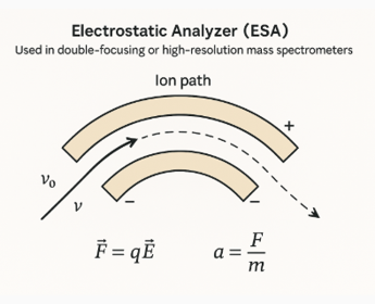
Electrostatic Analyzer (ESA)
An Electrostatic Analyzer is a key component in double-focusing or high-resolution mass spectrometers. Its primary purpose is to select ions based on their kinetic energy, thereby improving resolution by compensating for energy spread among ions of the same mass-to-charge ratio.
Structure: It consists of two curved electrodes that create a uniform radial electric field.
Operation: Ions enter the ESA and experience an electrostatic force that bends their trajectory. Only ions with the correct kinetic energy follow the designed circular path and exit toward the detector.
Basic Physics Behind ESA
The electrostatic force experienced by the ions inside the ESA is given by
where q is the ion’s charge and E is the electric field strength. This force acts as the centripetal force resulting in the ions circular path, giving
where m is the mass of the ion, v is the ion’s velocity and r is the radius of curvature. Combining the equations gives
You probably notice how closely these equation resemble the expression for kinetic energy. If we substitute for v, we get
This means that the ESA acts as an energy filter, allowing only ions with a specific kinetic energy to pass through.
Double-Focusing Mass Spectrometer
A double-focusing mass spectrometer combines two types of analyzers:
- A magnetic sector (which separates ions based on momentum)
- An electrostatic analyzer (ESA) (which selects ions based on kinetic energy)
This combination corrects for variations in both directional spread and energy spread of ions, leading to high resolution.
Principle of Double-Focusing
By carefully choosing the radii and angles of these sectors, ions of the same m/z converge at the detector, regardless of small initial energy or angular deviations.
Problem: When ions leave the ion source, they have slight differences in kinetic energy and angular direction. These variations cause broadening of the mass peak, reducing resolution.
Solution: Double-focusing uses two sectors:
- Magnetic sector: Bends ions according to their momentum (mv), so ions with the same m/z but different velocities follow slightly different paths.
- Electrostatic sector: Bends ions according to their kinetic energy (1/2 mv2), compensating for energy differences.
The magnetic sector corrects for angular spread and the ESA corrects for energy spread. Together, they ensure that ions of the same m/z arrive at the detector at the same point – this is double-focusing.
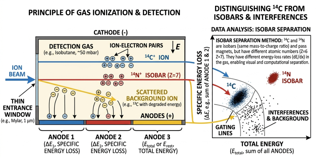
Gas Ionization Detector (GID)
A gas ionization detector in an AMS system measures the energy loss of incoming ions, allowing different isotopes to be distinguished even when their masses are similar. As energetic ions enter the detector, they first pass through a thin silicon nitride entrance window, which isolates the gas volume while allowing the ions to enter with minimal energy loss. Once inside the chamber, the ions collide with isobutane molecules, producing a cloud of ion–electron pairs along their tracks. The freed electrons drift toward a series of segmented electrodes arranged along the length of the gas cell. Because different ions produce different ionization profiles depending on their charge, mass, and energy, the pattern of charge collected on the segmented electrodes forms a characteristic “fingerprint” that the detector electronics use to uniquely identify the ion species.
Radiocarbon Applications (by material type)

Sample material categories are represented in the drop-down panels below and each panels contains a list of specific material types that can be radiocarbon dated.
Detailed information regarding the pretreatment methods necessary for many of these materials can be found on the Sample Information and Protocols page.
(For clarity, the last panel contains a list of materials that cannot be radiocarbon dated)
Plant-Derived Materials
Short‑lived plant tissues
- Seeds
- Nutshells
- Leaves
- Twigs
- Grass stems
- Reed fragments
- Pine needles
- Bark fragments
- Cones
Long‑lived plant tissues
- Wood
- Large branches
- Root fragments
Processed plant materials
- Paper
- Papyrus
- Textiles (cotton, linen, hemp, flax)
- Basketry
- Rope, cordage, twine
- Plant‑based adhesives or resins
- Charred food crusts on pottery
Animal-Derived Materials
Skeletal and hard tissues
- Bone
- Tooth dentin
- Tooth enamel (for carbonate dating)
- Antler
- Horn
- Ivory (mammoth, walrus, elephant)
- Tusk
- Insects (chitinous materials)
Soft tissues
- Skin
- Leather
- Hide
- Parchment
- Hair
- Fur
- Feather
- Hooves, Claws (keratinous tissues)
- Faeces
Biochemical extracts
- Bone collagen
- Gelatin
- Amino acid fractions (e.g., hydroxyproline)
Human-Derived or Related Materials
- Human bone
- Human teeth
- Hair
- Mummified tissue
- Faeces
- Cremated bone (carbonate fraction)
- Embalming resins
- Mortuary textiles
Marine, Freshwater and Aquatic Materials
Carbonate shells
- Marine mollusk shells
- Freshwater mussels
- Oyster, clam, scallop shells
- Snail shells (terrestrial or aquatic)
Other aquatic materials
- Coral
- Calcareous sponges
- Fish bone
- Fish otoliths
- Marine mammal bone
- Seaweed / kelp
- Algal mats
- Carbonate encrustations
Carbonate and Geological Materials
- Travertine
- Tufa
- Speleothems (limited applicability; often U‑series preferred)
- Carbonate crusts on artifacts
- Secondary carbonates in soils
Man-Made Materials
- Charred food residues on pottery
- Soot or lampblack
- Pitch, tar, bitumen (if biogenic)
- Mortar (if lime mortar with preserved atmospheric CO₂)
- Basketry and woven plant fibers
- Wooden tools or handles
- Canoe fragments
- Textile fragments
- Cordage and nets
- Glue or adhesive residues
- Resin coatings
- Paint binders (organic fraction)
- Historical paper documents
- Old textiles (clothing, flags, quilts)
- Wooden artifacts
- Leather goods
- Paintings (canvas, wood panel, organic binders)
- Wine, spirits, or food products (for authenticity testing)
- Tobacco, plant‑based drugs (for forensic provenance)
- Bio‑based plastics (to determine renewable vs. fossil carbon content)
Environmental Materials
Sediments & organics
- Peat
- Soil organic matter (SOM)
- Humic acids (with caution)
- Plant macrofossils
- Charred microfragments
- Lake sediment organic fractions
- Marine sediment organic fractions
Microfossils
- Pollen
- Phytoliths (if organic coatings preserved)
- Diatom organic residues
- Foraminifera (carbonate)
Other environmental materials
- Carbonates precipitated in aquatic systems
- Dissolved inorganic carbon (DIC) in water
- Dissolved organic carbon (DOC)
Materials that Cannot be Radiocarbon Dated
Why bother to list items that can’t be radiocarbon dated?
Well, people often ask about dating these materials without realizing that they either don’t contain any carbon or they are so old that all of the carbon-14 has decayed away.
Contain No Carbon
- Metals (iron, copper, gold, silver)
- Pure stone (granite, basalt, obsidian)
- Inorganic pigments
- Glass
- Fossils fully mineralized – no organic carbon left
No Carbon-14 Left (too old)
- Coal, oil, natural gas (radiocarbon-dead)
- Plastics and other materials made from petroleum
Radiocarbon Applications (by research discipline)
Archaeology
Non-Exhaustive List of Archeological Sample Types Suitable for Radiocarbon Analysis
- Charred food residues on pottery
- Soot or lampblack
- Pitch, tar, bitumen (if biogenic)
- Mortar (if lime mortar with preserved atmospheric CO₂)
- Basketry and woven plant fibers
- Wooden tools or handles
- Canoe fragments
- Textile fragments
- Cordage and nets
- Glue or adhesive residues
- Resin coatings
- Paint binders (organic fraction)
- Historical paper documents
- Old textiles (clothing, flags, quilts)
- Wooden artifacts
- Leather goods
- Paintings (canvas, wood panel, organic binders)
- Wine, spirits, or food products (for authenticity testing)
- Tobacco, plant‑based drugs (for forensic provenance)
- Bio‑based plastics (to determine renewable vs. fossil carbon content)
Paleontology
Non-Exhaustive List of Paleontological Sample Types Suitable for Radiocarbon Analysis
- Teeth
- Tusks
- Antlers
- Hair, fur, feathers
- Hooves, horns, claws
- Shells
- Foraminifera
- Coral skeletons
- Otoliths
- Insects
- Wood
- Charcoal
- Seeds
- Nut shells, pine cones
- Leaves, stems, grasses, sedges
- Roots
- Soil and sediment organic matter
Ecology
Non-Exhaustive List of Ecological Sample Types Suitable for Radiocarbon Analysis
- Peat
- Soil organic matter (SOM)
- Humic acids (with caution)
- Plant macrofossils
- Charred microfragments
- Lake sediment organic fractions
- Marine sediment organic fractions
- Pollen
- Phytoliths (if organic coatings preserved)
- Diatom organic residues
- Foraminifera (carbonate)
- Dissolved inorganic carbon (DIC) in water
- Dissolved organic carbon (DOC)
- Carbonates precipitated in aquatic systems
Geology
Non-Exhaustive List of Geological Sample Types Suitable for Radiocarbon Analysis
- Travertine
- Tufa
- Speleothems (limited applicability; often U‑series preferred)
- Pedogenic carbonates