Calculations and Results Format

We report radiocarbon measurement information in a format that our clients find the most useful and meaningful. However, there are some discrepancies between the reporting formats used by the various radiocarbon dating labs. Information is provided below regarding the results reporting format we use and also the various corrections we use (and the reasons for using them) when converting raw radiocarbon measurement data into usable ages.

Reported Data Format

Units and Conventions

Radiocarbon ages measured by AMS are reported using a fairly standardized set of conventions so results are comparable across labs, time, and calibration software. These conventions cover how the age is expressed (units, reference year, half-life), what corrections are applied, and how calibrated ages are distinguished from raw radiocarbon ages. A widely endorsed summary of these conventions was published by (Millard 2014) and has become the current reference point for best practice.

For additional details, please refer to the Radiocarbon Dating units and Conventions section of the Radiocarbon Dating Background Information page.

Age Reporting Format

Conventional radiocarbon age

The primary way to report an AMS result is as a conventional radiocarbon age, expressed as:

age \pm uncertainty\ ^{14}C\ yr\ BP

e.g.\ 3520 \pm 30\ ^{14}C\ yr\ BP

Unit: 14C yr BP or ¹⁴C yr BP (not just “years BP”).
BP definition: BP = “Before Present,” where “Present” is fixed as 1950 CE.
Half-life used: The Libby half-life of 5568 years is used for conventional ages, even though the more accurate physical half-life is 5730 years (Kondev 2021) this maintains compatibility with the historical radiocarbon scale.
Reference ratio: Ages are defined relative to a standard ¹⁴C/¹²C ratio that represents the atmosphere in 1950, assuming it was constant in the past (which is later corrected via calibration).
Uncertainty: Reported as one standard deviation (1σ), combining counting statistics and other quantifiable sources of error.

Fraction modern (F¹⁴C)

F¹⁴C is the isotope ratio of the sample normalized to a standard “modern” reference, corrected for isotopic fractionation, where: F¹⁴C = 1.0 represents the 1950 atmospheric level of ¹⁴C.

F^{14}C = 0.954 \pm 0.003

Dimensionless, but always explicitly labeled as F¹⁴C.

Usage: Particularly important for post‑bomb samples, modern carbon cycle, and ocean/atmosphere studies, where “age” in years is less intuitive or even ambiguous.

Millard’s conventions explicitly state that either a conventional age in ¹⁴C yr BP or an F¹⁴C value (or both) should be reported for each determination, with fractionation correction stated or implied.

Complete Result Report Breakdown

In line with Millard’s recommendations (Millard 2014), the following information is reported for every sample submitted.

AURORA Radiocarbon Dating Results Report Format

‘Section 0’

Intended as a ‘quick glance’ section… for those in a hurry.

Section 1 – Sample Details

Provides step-by-step information about the sample’s journey through the system, from initial inspection through pretreatment and all the way to analysis. This section also echoes the project, site and contextual information initially provided by the client.

Section 2 – Measurement Results

All measurement results are reported here – not just the AMS measurement. Extraction yields results and results from any form of prescreening (such as C:N) are reported here.

Section 3 – Age

Radiocarbon age and calibrated age are reported here along with their respective errors. Details regarding the calibration curve used and the calibration software that was used to perform the age calibration are also reported here.

Section 4 – Quality Assurance

The primary standards, secondary standards, process blanks and instrument blanks used are reported here.

Section 5 – Reporting Conventions Observed

This section contains a series of statements regarding the reporting conventions used in the report. It’s likely that clients will be left in no doubt that we use the most up-to-date and widely-accepted radiocarbon analysis reporting conventions, but just in case…

(Downloadable example Radiocarbon Dating Results Report coming soon)

Date Calibration (IntCal20, SHCal20, Marine20)

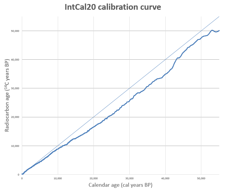
Raw AMS results (¹⁴C yr BP) do not directly equal calendar ages because atmospheric ¹⁴C has varied over time. Calibration curves and conventions for reporting calibrated ages are therefore crucial.

The plot below shows how the radiocarbon age has deviated from the calendar age.

Calibration curves

Current internationally accepted curves include:
- IntCal20 for the Northern Hemisphere.
- SHCal20 for the Southern Hemisphere.
- Marine20 for marine samples.

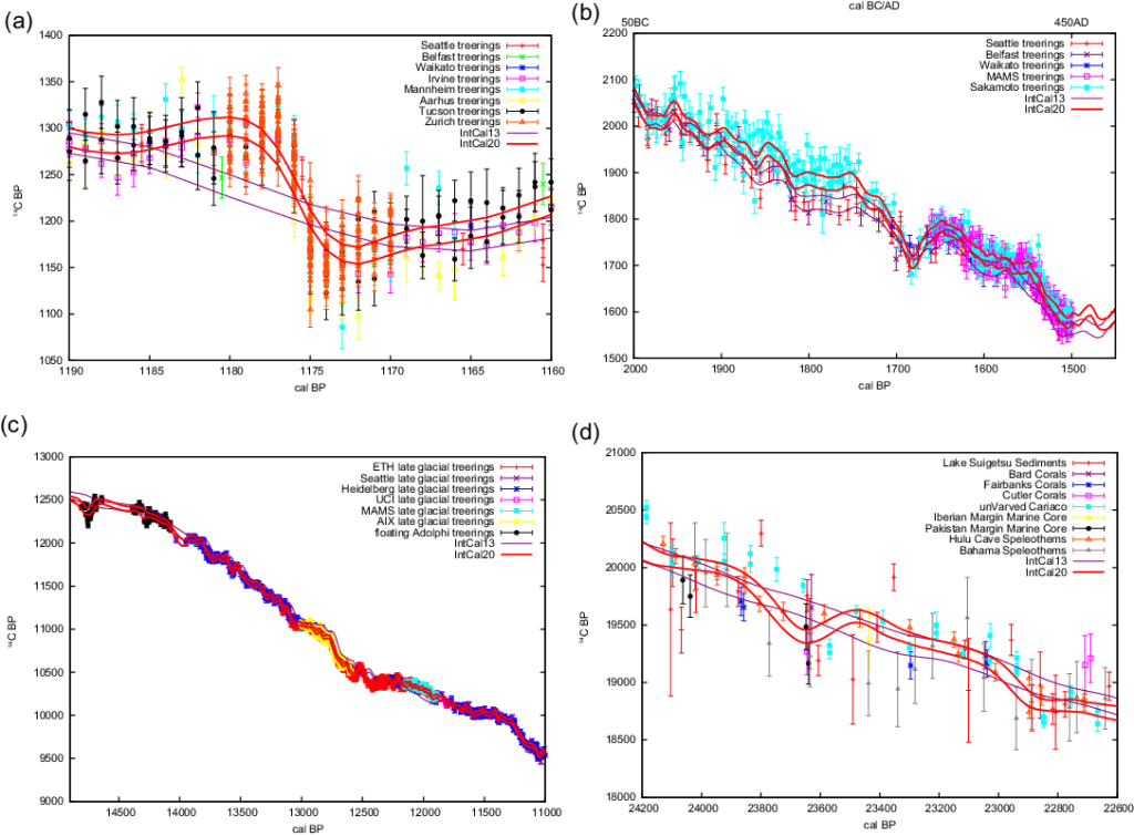
These curves are constructed from tree rings, corals, varves, and other archives, and are periodically updated.

The plots below clearly show how multiple chronology archives have been used to calibrate the atmospheric ¹⁴C concentration and provide a mean to correct the radiocarbon age.

Calibrated ages: formats and units

To avoid confusion between radiocarbon years and calendar years, clear distinctions in notation are used:

Calibrated ages in years before present:
- Format:
  cal BP or more explicitly “calibrated years BP”.
- Example:
  3820-3690 cal BP (95% probability, IntCal20)
Calendar years CE/BC (or AD/BC):
- Example:
  - 2460–2280 cal BCE (95% probability, IntCal20)
- “cal” is kept to indicate the age is calibrated, and the curve used should be stated.
Key convention:
Millard notes that earlier conventions did not formally cover calibrated dates, and his updated guidelines explicitly recommend clearly distinguishing between conventional radiocarbon ages (¹⁴C yr BP) and calibrated calendar ages (cal BP, cal CE/BCE), and always stating which calibration curve and software were used.

Calculations and Corrections

All measurements performed on the MiCaDaS use BATS (Beautiful AMS Tool of Switzerland) developed at ETH Zurich by Lukas Wacker and colleagues (Wacker 2010). BATS was specifically designed to meet the analytical and operational needs of compact AMS systems like MiCaDaS. BATS provides automated, standard‑ and blank‑corrected results with minimal user input, making data reduction both efficient and highly reproducible. Its underlying algorithms were built to handle MiCaDaS measurement formats directly, ensuring that corrections, normalization, and uncertainty propagation are applied consistently and according to instrument‑specific behavior. After extensive routine operation on MiCaDaS systems, BATS has proven to be a robust, user‑friendly, and reliable tool for generating high‑quality radiocarbon results. This tight integration between the software’s design philosophy and the MiCaDaS measurement workflow makes BATS the natural choice for processing our raw AMS data.

Calculations and Corrections Applied to All Samples (using BATS)

Raw Isotope Ratios from the AMS Detectors

In the MiCaDaS AMS (Synal 2007), ¹²C and ¹³C currents are measured in Faraday cups, while ¹⁴C is counted in a gas ionization detector. These signals are integrated over time to give time‑averaged count rates or currents for each isotope. The basic ratio is then computed by BATS as

R_{raw}=N(^{14}C)/N(^{12}C)

At this stage, the ratio is still “instrumental”: it reflects whatever fractionation, contamination, and instrumental bias is present, and has not yet been referenced to a standard or corrected for blanks or isotopic composition.

Note: It’s convenient to consider that this raw ratio has not undergone any corrections yet, but in reality several corrections have already been applied by the MiCaDaS instrument itself. The Faraday cup measurements are strongly influenced by amplifier characteristics including offset, gain, noise and response-time (Tau). The carbon-14 gas ionization detector measurements are similarly affected by gain, noise, and dead-time. All AMS instruments employ sophisticated electronic methods to negate or minimize the negative effects of these characteristics, in essence employing ‘electronic’ corrections.

¹⁴C⁺ Background Subtraction (¹³CH⁺ Contribution) [Deprecated]

The design of accelerator mass spectrometers is such that there are very few ions other than ¹⁴C⁺ that can reach the gas ionization detector and directly interfere with the ¹⁴C measurement. The methylidyne ion of ¹³C (¹³CH⁺) is formed in small quantities in the stripper canal of the accelerator as a result of the break up of organic molecules. The MiCaDaS (ref) uses an additional Faraday cup detector after the high energy magnet to detect the ¹³C⁺ resulting from broken up carbon-containing molecules(¹³C_mol). There is a linear correlation between the detected ¹³C⁺ from broken up molecules and the ¹³CH⁺ ion that reaches the gas ionization detector. BATS can employ a correction factor (k_mol) to subtract the interfering ¹³CH⁺ background from the ¹⁴C ion count.

R_{mol}=\frac{N(^{14}C)-(k_{mol}*N(^{13}C_{mol}))}{N(^{12}C)}

This correction was employed when nitrogen was used as the stripper gas. When the MiCaDaS stripper design was changed to utilize helium as the stripper gas, the methylidyne ion formation dropped precipitously and is no longer considered to be a significant source of error. This correction is no longer routinely enabled in BATS.

Blank Correction

In radiocarbon dating, the blank represents the apparent ¹⁴C signal that is measured when analyzing material that should contain no ¹⁴C at all. In other words, it reflects all sources of extraneous carbon and spurious ¹⁴C introduced during sample preparation, handling, measurement, and data processing, rather than carbon intrinsic to the sample. Because AMS is capable of detecting ¹⁴C/¹²C ratios at the level of 10⁻¹⁵–10⁻¹⁶, even extremely small contaminant contributions can significantly bias results, especially for old or small samples.

Practically, the blank defines the maximum measurable age, the background level, and the ultimate precision limit of an AMS laboratory. Blank correction is therefore central to all high‑quality radiocarbon measurements.

For more information about the blank, take a look at this section of the radiocarbon dating background information page.

BATS takes the weighted mean of all the measured blanks in the magazine or sample tray $\langle R(bl)_{mol} \rangle$ and subtracts it from all the samples and standards in the magazine or sample tray

R_{bl}=R-\langle R(bl) \rangle

This correction is employed under the assumption that all the sample and standard sizes are the same.

Weighted mean values are used throughout by BATS

\langle X \rangle =\sum_{i}^{}\frac{X_{i}*p_{i}}{\sum_{i}^{}p_{i}}

where the weight of a single measurement p_i is the ¹²C charge during the measurement of ¹⁴C. This is calculated from the current multiplied by the time

charge = current * time p_i = ¹²C current * collection time

Note: If it’s necessary to run samples of differing sizes, then the default blanks subtraction in BATS will be disabled and a more sophisticated blank correction used that scales the size of the mean blank to correspond with the size of the sample (using a mass balance equation – see the small sample section).

Fractionation Correction

Fractionation results from almost every stage of the radiocarbon dating process, but the largest fractionation effects are produced by the AMS. The main factors are the negative ion formation in the ion source (Nadeau 1987), the stripping efficiency (Finkel 1993), and the ion-optical transmission through the whole machine. The measured ¹³C/¹²C is used by BATS to calculate the δ¹³C and then correct the ¹⁴C/¹²C by assuming that the fractionation effect for ¹⁴C is twice that of ¹³C and the global average δ¹³C is -25‰ . Since the ionization and ion beam focus conditions are continually changing as the sample graphite is consumed, every measurement must be corrected for fractionation. BATS calculates the weighted mean of the measured ¹³C/¹²C of all standards in the magazine or sample tray with a given δ¹³C_std $\langle (^{13}C /^{12}C)_{std} \rangle$ . Then the single measurement δ¹³C is calculated (in units of permil ‰)

\delta^{13}C=\left[ \frac{(^{13}C/^{12}C)*(1+\delta^{13}C_{std}/1000)}{\langle (^{13}C /^{12}C)_{std} \rangle}-1 \right]*1000

R_bl of the single measurement is then corrected for fractionation

R_{bl,f}=R_{bl}*\left(\frac{0.975}{1+\delta^{13}C/1000} \right)^2

Note: the fractionation correction is typically the largest correction employed and has a substantial impact on radiocarbon measurement precision.

Correction to the Primary Standard

HOxI and HOxII (hydrogen oxalate I and II, otherwise known as oxalic acid I and II) are the only primary radiocarbon standards. Secondary standards, such as ANU Sucrose have been carefully calibrated against HOxI or HOxII. Primary or secondary standards are routinely analyzed alongside samples so that ¹⁴C/¹²C ratio offsets can be corrected. BATS calculates the weighted mean of all fractionation-corrected standard measurements $\langle R(std)_{bl,f} \rangle$ is calculated and then the background-, blank- and fractionation-corrected ratios R_bl,f of all samples are corrected to the primary standard

R_{bl,f,std}=\frac{R_{nom}}{\langle R(std)_{bl,f} \rangle}*R_{bl,f}

where R_nom is the nominal fraction ¹⁴C value of the standard (Reimer 2004).

Note: while not the last of the calculations, this is the end of the corrections performed by BATS. BATS next calculates the weighted sample means of the corrected individual measurements – typically, 10 ‘passes’ are performed on each sample, that is there are 10 individual measurements on each sample. After that, BATS calculates the compounded errors to establish the overall uncertainty of the measurement.

Sample Means

Since each sample undergoes multiple individual measurements (typically 10 ‘passes’ for each sample), the next step that BATS performs is to calculate the weighted means for each sample $\langle R_{bl,f,std} \rangle$ and similarly the mean δ¹³C for each sample.

\langle R_{bl,f,std} \rangle=\frac{\sum_{i}^{}((R_{bl,f,std})_i*p_i)}{\sum_{i}^{}p_i}

\langle \delta^{13}C \rangle=\frac{\sum_{i}^{}((\delta^{13}C)_i*p_i)}{\sum_{i}^{}p_i}

Uncertainty (Error)

First, the uncertainty of the counting statistic N(¹⁴C) is calculated for a single measurement:

\sigma_{R}=\sqrt{N(^{14}C)+\left(N(^{13}C) \right)^2}

The uncertainty for the sample mean is given by

\sigma_{\langle R \rangle}=\frac{\Sigma_{i} \left( (\sigma_{R})_i*p_i\right)}{\Sigma_ip_i}

Next, the variability of the blank samples $\langle R \rangle_i$ is accounted for

\sigma_{ \langle R(bl) \rangle}=\frac{\Sigma_i \left( \langle R \rangle_i- \langle R(bl) \rangle \right)^2}{n-1}

The blank scatter uncertainty is added and corrected for fractionation

\sigma_{R_{bl,f}}=\sqrt{\sigma_{\langle R \rangle}^2+\sigma_{\langle R(bl) \rangle}^2}* \left( \frac{0.975}{1+ \langle \delta^{13}C \rangle /1000} \right)^2

That takes care of the theoretical uncertainty, but unfortunately the true uncertainty of the measurement is greater than that. To provide a better estimate of the true uncertainty, BATS adds an ‘external’ error that is estimated from the Micadas’ performance under normal and stable measurement conditions. See Wacker 2010 for a more detailed explanation of how this external uncertainty σ_ex is derived.

\sigma_{R_{bl,f,ex}}=\sqrt{\sigma_{\langle R_{bl,f} \rangle}^2+\sigma_{ex}^2}

Finally, BATS accounts for the uncertainty introduced by the correction to the standards. The uncertainty of the weighted mean of all standards is

\sigma_{ \langle R(std)_{bl,ex} \rangle}=\frac{\Sigma_s \left( \left( \sigma_{R_{bl,f,ex}} \right)_s * p_s \right)^2}{p_s}

and the final calculation combining all sources of uncertainty is

\sigma_{\langle R_{bl,f,ex,std} \rangle}=\langle R_{bl,f,std} \rangle * \sqrt{\left( \frac{\sigma_{\langle R_{bl,f,ex} \rangle}}{\langle R_{bl,f} \rangle } \right)^2+\left( \frac{\sigma_{\langle R(std)_{bl,f,ex} \rangle}}{\langle R(std)_{bl,f} \rangle } \right)^2+\left( \frac{\sigma_{ R_{nom}}}{ R_{nom}} \right)^2}

Note: for higher precision measurements, σ_ex is estimated directly from an increased number of standards measured together with the samples.

Fraction Modern (F¹⁴C)

Fraction Modern (F¹⁴C) is the fundamental, dimensionless unit defined in the modern radiocarbon standardization system. It is the ratio of a sample’s ¹⁴C/¹²C (normalized to δ¹³C = –25‰) to the internationally defined “modern” reference (Oxalic Acid I, normalized to 1950). F¹⁴C values therefore range from 0 (no detectable ¹⁴C) upward, with bomb‑pulse samples often exceeding 1.0.

Because radiocarbon ages are defined in years “before present” (BP), where “present” is conventionally 1950, measurements made in other years must account for the additional decay that occurred between 1950 and the measurement date. If the laboratory measures a fraction modern relative to a contemporary standard at measurement year (t_m), and wants F¹⁴C referenced to 1950, the value is adjusted using the decay law with the mean life (tau = 8033) years corresponding to the Libby half‑life of 5568 years:

F^{14}C=F_{meas}*e^{(t_m-1950)/ \tau}

This effectively “back‑decays” the measured fraction to what it would have been in 1950, so that a sample fixed in 1950 atmosphere and measured decades later still has F¹⁴C of approximately 1 after correction

Conventional Radiocarbon Age

The radioactive decay law is used to convert F¹⁴C into a conventional radiocarbon age. Radiocarbon ages are defined using the Libby half‑life of 5568 years, even though the actual physical half‑life is 5730 years (Kondev 2021), to preserve comparability with the historical radiocarbon literature. Using the decay constant $\lambda=ln(2)/5568$ or equivalently the mean life $\tau=8033$ years, the conventional age (t) is

t=- \tau ln(F^{14}C)=-8033ln(F^{14}C)

The result is reported as an age in years BP (before 1950), e.g. (4320 ± 40) ¹⁴C yr BP, with the uncertainty propagated from counting statistics, blank, standard, and fractionation corrections (see the above uncertainty section). This “conventional radiocarbon” age is deliberately idealized, it assumes a constant ¹⁴C production rate and atmospheric concentration equal to that of 1950, and it uses a fixed half‑life, which is why it must normally be calibrated before being treated as a calendar age.

Note: percent modern (pM) or percent modern carbon (pMC) is simply a scaled version of Fraction Modern pMC=100*F¹⁴C. Historically, pMC was widely used in reporting radiocarbon results because it is intuitive: 100 pMC corresponds to modern carbon (F¹⁴C = 1.0), values >100 pMC indicate bomb‑radiocarbon enrichment, and values <100 pMC reflect radioactive decay. However, pMC is essentially just a percentage expression of F¹⁴C, and F¹⁴C is now preferred in scientific publications because it is directly tied to standardized definitions, calibration, and statistical treatment.

Calculations, Corrections and Calibrations Applied Selectively

Reservoir Corrections

In many applications, a further correction is applied for reservoir effects before calibration. If the carbon source was not in instantaneous equilibrium with the atmosphere (e.g., marine carbon, lake systems with hard‑water effects, or old groundwater), the apparent ¹⁴C age will be offset from the true formation age by a reservoir age. This is often parameterized as $\Delta R$ or specific reservoir age corrections derived from paired ¹⁴C–calendar dated materials in the same reservoir. Mathematically, this is usually expressed as a simple adjustment to the conventional age, e.g.

t_{corr}=t_{conventional}- \Delta R

with the associated uncertainty added in quadrature. Conceptually, you are saying: “given what we know about this reservoir’s baseline offset from the atmosphere, what age would this measurement correspond to if it had been atmospheric?” This corrected age is then what proceeds to calibration.

Calibration to Calendar Age

Finally, to convert the conventional radiocarbon age into a usable calendar age, the age must be calibrated against an independently dated record of atmospheric (or reservoir‑specific) ¹⁴C history. Tree‑ring sequences, corals, varves, and other archives have been used to reconstruct how atmospheric ¹⁴C has varied over time; this information is codified in calibration curves such as IntCal, Marine, and others. Calibration software (e.g., OxCal or similar) takes the conventional age and its uncertainty and maps it onto the calibration curve using Bayesian or probabilistic methods, yielding a probability distribution in calendar years rather than a single point estimate. The output is typically given as ranges like “cal BP” or calendar BCE/CE with specified probabilities (e.g., 95.4%), which is what most users treat as the “usable age” in archaeological and geoscience interpretations. The calibration step does not change the underlying measurement; it reinterprets that measurement in the context of known temporal variations in ¹⁴C production and carbon cycling.

IntCal20 Calibration

Radiocarbon ages derived directly from AMS measurements must be calibrated because atmospheric ¹⁴C concentrations have varied substantially through time. IntCal20 is the most recent internationally ratified calibration curve for the Northern Hemisphere, extending from the present back to 55,000 calibrated years BP. It was constructed by the IntCal Working Group using a wide range of independently dated archives—including tree rings, corals, speleothems, and marine and lacustrine sediments—to quantify past fluctuations in atmospheric ¹⁴C levels and convert radiocarbon years into true calendar ages (Reimer 2020). When a laboratory obtains a radiocarbon age (e.g., 3,500 ± 30 ¹⁴C yr BP), that age is mapped onto the IntCal20 curve to determine the range(s) of calendar years that correspond to the measured ¹⁴C value. Calibration software such as OxCal or Calib uses IntCal20’s dataset of ¹⁴C ages and uncertainties to produce a probability distribution of possible calendar ages. IntCal20 is freely available for download from the official IntCal website at https://www.intcal.org and from academic repositories such as Cambridge University Press and data packages such as the IntCal R library.

SHCal20 Calibration

Radiocarbon ages derived directly from AMS measurements must be calibrated because atmospheric ¹⁴C concentrations have varied substantially through time. SHCal20 is the most recent internationally ratified calibration curve for the Southern Hemisphere, extending from the present back to 55,000 calibrated years BP. It was constructed by the IntCal Working Group using a wide range of independently dated archives—including tree rings, corals, speleothems, and marine and lacustrine sediments—to quantify past fluctuations in atmospheric ¹⁴C levels and convert radiocarbon years into true calendar ages (Hogg 2020). When a laboratory obtains a radiocarbon age (e.g., 3,500 ± 30 ¹⁴C yr BP), that age is mapped onto the IntCal20 curve to determine the range(s) of calendar years that correspond to the measured ¹⁴C value. Calibration software such as OxCal or Calib uses SHCal20’s dataset of ¹⁴C ages and uncertainties to produce a probability distribution of possible calendar ages. SHCal20 is freely available for download from the official IntCal website at https://www.intcal.org and from academic repositories such as Cambridge University Press and data packages such as the IntCal R library.

Marine20 Calibration

Marine20 is the internationally accepted radiocarbon calibration curve for marine samples, developed by the IntCal Working Group to correct radiocarbon ages for the unique behavior of ¹⁴C in the global ocean system. Because the ocean mixes much more slowly than the atmosphere, marine dissolved inorganic carbon can be several hundred years “older” than atmospheric carbon, and this offset varies through time and by region. Marine20 provides a statistically integrated record of past marine ¹⁴C levels based on independently dated archives—including corals, foraminifera, and sediment cores—and applies improved modeling of marine reservoir ages using a three‑dimensional ocean circulation model rather than relying on fixed regional offsets (Heaton 2020). When calibrating a reported radiocarbon age, software such as OxCal or Calib uses Marine20 to convert measured ¹⁴C years into calendar ages while incorporating location‑specific reservoir corrections (ΔR). Marine20 is freely available for download on the official IntCal data site at https://www.intcal.org/curves.html, which hosts the full datasets and metadata for all IntCal20‑series calibration curves.

OxCal and Calib Calibration Programs

OxCal and Calib are both widely used radiocarbon calibration programs, but they differ significantly in purpose, capabilities, and underlying statistical approaches. Calib, originally developed by Stuiver and Reimer, is designed primarily for straightforward radiocarbon calibration, converting ¹⁴C ages to calendar ages using published calibration curves—its focus is simplicity, direct age–curve interpolation, and standardized reporting of calibrated ranges. OxCal, developed by Christopher Bronk Ramsey at the Oxford Radiocarbon Accelerator Unit, includes all the basic calibration functions but is also a full Bayesian chronological‑modeling environment. It allows users to incorporate stratigraphic relationships, sequence models, phase boundaries, wiggle‑matching, reservoir corrections, and probability‑based evaluation of entire chronological frameworks, going far beyond simple calibration. OxCal uses Bayesian statistical methods and Monte‑Carlo sampling (Gibbs sampling) to integrate radiocarbon measurements with archaeological or geological prior information, producing probability distributions that reflect both the ¹⁴C data and the structure of the model supplied by the user. Calib, in contrast, does not implement Bayesian modeling and is focused on individual-date calibration rather than analysis of complex sequences. Both programs use the same IntCal‑series calibration curves, and both support marine and mixed calibrations, but OxCal provides much more flexibility for advanced chronological research.

Access OxCal here and the program manual here.

Access Calib here and the program manual here.

Small Samples

Error and Uncertainty

This section is intended to provide some additional background in case some of the mathematical gymnastics in the Calculations and Corrections section above were unfamiliar.

Measurement Errors

Measurement error is the difference between the actual (true) value of a quantity and the value recorded during a measurement. In the context of radiocarbon measurements, the measurement error is the difference between the actual amount of carbon-14 present in a sample and measured amount of radiocarbon present in the sample.

Measurement errors consist of systematic errors and random errors. Again, in the context of our radiocarbon measurements, systematic errors are eliminated when we apply corrections using primary and secondary standards – we know the amount of carbon-14 present in these materials and with that knowledge we can identify and correct systematic offsets. Random errors are unpredictable, naturally occurring variations that fluctuate above and below the true value. Since it’s impossible to exactly quantify random errors, we quantify the possible effect of the errors and express the outcome as an uncertainty.

Measurement Uncertainty

Measurement uncertainty is the inherent doubt or margin of error associated with any measurement. It quantifies the dispersion of values that could reasonably be attributed to the true value.

In the Calculations and Corrections section above, the statistically-derived theoretical uncertainty is calculated. Since this uncertainty is derived from processes occurring inside the MiCaDaS AMS, it’s referred to as the ‘Internal Uncertainty’ (although not strictly correct, uncertainty is often referred to as ‘error’ – potentially confusing, but common practice). External uncertainty is the dispersion of values that could reasonably be attributed to the ‘true value’ and is obviously subject to different interpretations. A meaningful assessment of external uncertainty must account for the errors introduced during sample pretreatment and preparation. Our practice is to assess external uncertainty by using the dispersion of values obtained for our secondary standards when possible. This approach depends critically on having a wide range of material types represented by our standards and having sufficient data points to provide robust statistical values.

Internal Uncertainty (Error) and Propagation Rules

Counting uncertainty, also called Poisson or statistical error is the inherent uncertainty in measuring random, independent events (like carbon-14 ion detection). Because the events are random, the best estimate of the standard deviation (σ) is simply the square root of the total number of recorded counts (N).

When mathematically processing our raw data, the uncertainty must be processed accordingly using the rules of error or uncertainty propagation. Counting (Poisson) uncertainty grows like the square root of counts and we propagate it by adding variances for sums/subtractions and adding relative variances for products/divisions. This means that averaging reduces random uncertainty by √N, while subtracting blanks and normalizing to standards increase the relative contribution of each component’s uncertainty to the final result.

Basic Propagation Rules

Sum or difference (z=x ± y): variances add

\sigma_z=\sqrt{\sigma_x^2+\sigma_y^2}

Product or ratio (z=x . y) or (z=x / y): relative variances add

\left(\frac{\sigma_z}{z}\right)=\sqrt{\left(\frac{\sigma_x}{x}\right)^2+\left(\frac{\sigma_y}{y}\right)^2}

Worked Simplified Radiocarbon Example

1. Single measurement (raw counts)

Sample:\\ (N_s=10{,}000) counts → (\sigma_s=\sqrt{10{,}000}=100)

Blank:\\ (N_b=400) counts → (\sigma_b=\sqrt{400}=20)

2. Subtract blank (net counts)

(N_{\text{net}}=N_s-N_b=9{,}600)

Propagate:\\ \sigma_{\text{net}}=\sqrt{\sigma_s^2+\sigma_b^2}=\sqrt{100^2+20^2}=\sqrt{10{,}400}\approx102

Relative\ uncertainty:\\ \sigma_{\text{net}}/N_{\text{net}}\approx102/9600\approx1.06%

3. Averaging repeated measurements

If you repeat the sample measurement (n=4) independent times and take the mean, the standard error of the mean is:

\sigma_{\bar N}=\frac{\sigma_{\text{single}}}{\sqrt{n}}=\frac{100}{2}=50

If the blank is also averaged (4 repeats) with σ_blank=20/2=10, then after subtraction the net mean uncertainty is:

\sigma_{\text{net,mean}}=\sqrt{50^2+10^2}=\sqrt{2{,}600}\approx51

Averaging therefore reduced the sample contribution from 100 to 50, and the net uncertainty from 102 to ≈51 (about half).

4. Correction to a standard (division)

Suppose a standard run gives:

N_{\text{std}}=20{,}000\\ with\\ \sigma_{\text{std}}=\sqrt{20{,}000}\approx141.4

The normalized ratio is:

R=N_{\text{net}}/N_{\text{std}}

The relative uncertainty in R is:

\frac{\sigma_R}{R}=\sqrt{\left(\frac{\sigma_{\text{net}}}{N_{\text{net}}}\right)^2+\left(\frac{\sigma_{\text{std}}}{N_{\text{std}}}\right)^2}

Using the averaged net example:

N_{\text{net}}=9{,}600,\ \sigma_{\text{net}}\approx51

\frac{\sigma_R}{R}=\sqrt{(51/9600)^2+(141.4/20000)^2}

\approx\sqrt{(0.0053)^2+(0.00707)^2}\approx0.0088\ (0.88\%)

External Uncertainty (Error)

We consider that the more accurate assessment of our uncertainty is provided by the spread of our results for primary and secondary standards. The spread of values obtained for a bone standard for example includes the errors associated with the pretreatment, preparation and radiocarbon measurement and this is the most reliable way to assess uncertainty for a bone sample that has undergone exactly the same processes. In the absence of appropriate standard data, the ‘external error’ estimation provided by BATS gives the most reasonable estimate of the average external uncertainty based on large numbers of analyses (see the Corrections and Calculations section above).

AURORA Lab

Institute of Northern Engineering

Calculations and Results Format

Units and Conventions

Age Reporting Format

Complete Result Report Breakdown

AURORA Radiocarbon Dating Results Report Format

Date Calibration (IntCal20, SHCal20, Marine20)

Calculations and Corrections Applied to All Samples (using BATS)

Raw Isotope Ratios from the AMS Detectors

¹⁴C⁺ Background Subtraction (¹³CH⁺ Contribution) [Deprecated]

Blank Correction

Fractionation Correction

Correction to the Primary Standard

Sample Means

Uncertainty (Error)

Fraction Modern (F¹⁴C)

Conventional Radiocarbon Age

Calculations, Corrections and Calibrations Applied Selectively

Reservoir Corrections

Calibration to Calendar Age

IntCal20 Calibration

SHCal20 Calibration

Marine20 Calibration

OxCal and Calib Calibration Programs

Small Samples

Measurement Errors

Measurement Uncertainty

Internal Uncertainty (Error) and Propagation Rules

Basic Propagation Rules

Worked Simplified Radiocarbon Example

External Uncertainty (Error)

Calculations and Results Format

Units and Conventions

Age Reporting Format

Complete Result Report Breakdown

AURORA Radiocarbon Dating Results Report Format

Date Calibration (IntCal20, SHCal20, Marine20)

Calculations and Corrections Applied to All Samples (using BATS)

Raw Isotope Ratios from the AMS Detectors

14C+ Background Subtraction (13CH+ Contribution) [Deprecated]

Blank Correction

Fractionation Correction

Correction to the Primary Standard

Sample Means

Uncertainty (Error)

Fraction Modern (F14C)

Conventional Radiocarbon Age

Calculations, Corrections and Calibrations Applied Selectively

Reservoir Corrections

Calibration to Calendar Age

IntCal20 Calibration

SHCal20 Calibration

Marine20 Calibration

OxCal and Calib Calibration Programs

Small Samples

Measurement Errors

Measurement Uncertainty

Internal Uncertainty (Error) and Propagation Rules

Basic Propagation Rules

Worked Simplified Radiocarbon Example

External Uncertainty (Error)

¹⁴C⁺ Background Subtraction (¹³CH⁺ Contribution) [Deprecated]

Fraction Modern (F¹⁴C)